Tableau - Exploring Cohort Analysis
Tableau - Cohort Analysis

Simply put, cohort analysis is a technique for analyzing activity over time by a common characteristic. Mostly used in sales and marketing, cohort analysis can be used in tasks such as analyzing customer loyalty, customer cost acquisition, marketing campaign effectiveness and to explore many other aspects of sales.
Dataset
I am using the superstore sales created by Michael Martin found here or here. This excel file contains three sheets of which only the first one, Orders, will be used in this analysis.
Case
The store providing their sales data does monthly advertising campaigns and wants to track what impact these advertising campaigns have on the amounts of orders placed over time. They want to use this information to evaluate their different campaigns and improve their efforts.
Given the superstore sales data and the requirements, lets present the number of orders placed per customer join date. Presenting the number of orders per join date will show the effectiveness of advertising campaigns leading to such date.
Tools
Any database server can be used to follow along. The code used here can easily be revised to work on any vendor’s product like MySQL, etc. For visualization purposes, Tableau can be easily changed replaced by LibreOffice or similar.
Analysis
From the Orders Sheet, we are only going to use the following columns: Order Id, Order Date and Customer Name. For further analysis, however, lets preserve all the data in our system by saving the contents of the Orders Sheet in a database table.
Lets appropriately call this table superstore_sales. Also, lets execute our analysis for month/year to match the store’s advertising efforts.
-
First, lets fetch the orders, together with the order date and the customer name.
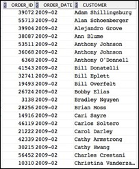
 select
 	a.order_id
 	, to_char(a.order_date, 'YYYY-MM') order_date
 	, a.customer_name customer
 from
 	superstore_sales a
 group by
 	a.order_id, a.order_date, a.customer_name
 order by 2,3;
-
To this set, lets add the date each customer placed their first order in the store.
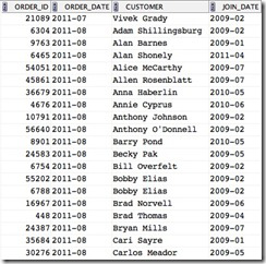
 select
 	a.order_id
 	, to_char(a.order_date, 'YYYY-MM') order_date
 	, a.customer_name customer
 	, to_char(min(b.order_date), 'YYYY-MM') join_date
 from
 	superstore_sales a
 inner join
 	superstore_sales b on a.customer_name = b.customer_name
 group by
 	a.order_id, a.order_date, a.customer_name
 order by 2,3;
-
Interested in the effect of each month’s advertising campaign, lets create a campaign id for each month. Basically, join date becomes campaign id. Notice we dropped the customer name as well. This is our join criteria only at this point.
Here we see, for each order placed, the monthly campaign to attribute the order to. Neat.
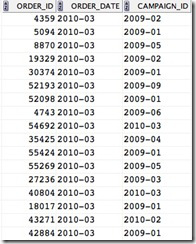
 select
 	a.order_id
 	, to_char(a.order_date, 'YYYY-MM') order_date
 	, to_char(min(b.order_date), 'YYYY-MM') campaign_id
 from
 	superstore_sales a
 inner join
 	superstore_sales b on a.customer_name = b.customer_name
 group by
 	a.order_id, a.order_date, a.customer_name
 order by 2;
-
Now, lets determine the number of months between the join date for each order’s customer first order and the order date for each order.
This is a mouthful; lets explain. It is easier to see it if explained backwards.
For each customer, calculate the number of months between their first order and every other order they have placed.
There, this makes a bit more sense.
Now we have a set of all orders by date by campaign and the number of months since the customer joined store.
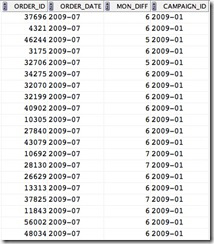
 select
 	a.order_id
 	, to_char(a.order_date, ‘YYYY-MM') order_date
 	, round(months_between(a.order_date,min(b.order_date))) mon_diff
 	, to_char(min(b.order_date), ‘YYYY-MM') campaign_id
 from
 	superstore_sales a
 inner join
 	superstore_sales b on a.customer_name = b.customer_name
 group by
 	a.order_id, a.order_date
 order by 2, 4;
-
Next up, we simply count orders by campaign id by number of months since customer joined store.
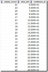
 select
 	count(distinct order_id) order_count,
 	mon_diff,
 	campaign_id
 from (
 	select
 		a.order_id
 		, round(months_between(a.order_date,min(b.order_date))) mon_diff
 		, to_char(min(b.order_date), ‘YYYY-MM') campaign_id
 	from
 		superstore_sales a
 	inner join
 		superstore_sales b on a.customer_name = b.customer_name
 	group by
 		a.order_id, a.order_date
 	order by 1
 	)
 group by
 	mon_diff, campaign_id
 order by campaign_id;
This is enough to satisfy our case; not bad. Now we have the set we need to analyze sales by campaign id over time. A short dive into Tableau (try Public) and we come out with an elegant way to view a lot of information at once.
Lets go over the visualization together.
The y axis represents the number of sales (order count), the x axis represents how many months ago (months diff) these sales occurred and the different colors each represent a campaign (campaign id).
Using the first month (ago) as an example, we can tell how many orders can be attributed to each campaign for the life of the data set. Skipping to the last month, 48, we see how many orders were placed for the campaign that occurred back then. Seeing only one color makes sense since that is our first advertising campaign.
The interactive version of the visualization above is here for you to try. There, you can see the actual numbers of orders per campaign, etc.
That’s it; thanks for reading. This seems like a very effective way to analyze a large amount of sales data for insights into advertising performance.
This post only covers join date as the grouping characteristic; many other cases can be made where cohort analysis can be helpful. Similarly, many other visualizations can provide similar insight.
Maybe next time we can cover some of these; thanks for reading!